Interest Rate Term Structure
The purpose of this document is to provide an overview of the risk-free rate curves used by SpiderRock Connect. There are now 3 different rate curves (OIS, Libor, and SpxBox), and they are stored and updated in the SRSE SRAnalytics table under msgGlobalRates. All three rate curves are outlined in this document.
The default SpiderRock term structure has been updated to use SPX box market prices to determine the risk-free interest rates which are implied directly from the option markets. In the past, SpiderRock market rates have been manually updated by taking the latest posted LIBOR rates and extrapolating longer-dated term rates from the US Treasury yield curve rates. In a low rate environment, the risk-free rate has been relatively insignificant as a pricing input, but as interest rates have increased, they have become more relevant, particularly for longer-dated options.
Fed Funds Futures and OIS Rates
An Overnight Index Swap (OIS) is an interest rate swap where the floating leg of the swap is equal to the geometric average of the overnight cash rate over the swap period. Overnight lending involves little default or liquidity risk; hence the fed funds futures, which correspond to the average delivered fed funds rate over each month, can be used to approximate this rate.
For a given term in days, D, the price of a zero-coupon bond can be approximated from the fed funds futures prices covering the months over the rate period. Suppose 𝐹𝐹1 corresponds to the front fed funds futures, 𝐹𝐹𝑛 corresponds to the fed funds futures contract which covers the final day of the rate period, and 𝑑𝑖 corresponds to the number of days in each month covered by the term so that 𝐷 = Σ𝑛𝑖=1𝑑𝑖. The zero-coupon bond price can then be calculated as:
Using the fed funds futures, we can calculate a term structure out to 2 years, and we can extrapolate further using the rate from the longest maturity in the fed funds futures.
Eurodollar and LIBOR Rates
A commonly used source for building a term structure from LIBOR market rates is the Eurodollar futures markets. The futures markets are highly liquid, and the markets cover the entire term structure needed for traded options.
Forward Rate from Eurodollar Futures
The Eurodollar futures rates differ from the corresponding market forward rates covering the same timeframe because futures contracts involve daily cashflows to account for changes in the rate environment, whereas forward rate instruments do not. The difference is minimal for short-dated contracts (e.g. less than a year), but for longer-dated maturities, a “convexity adjustment” should be used.
For SpiderRock interest rates, we choose to apply the Ho-Lee convexity adjustment formula:
where is the time to maturity of the futures contract, is the time to maturity of the forward rate underlying the futures contract, and the short rate volatility (𝜎) is taken from the Eurodollar option markets by interpolating a 1-year volatility of the 3-month futures rate from SpiderRock's ATM term structure.
Stub Rates
Standard practice for generating term rates from quarterly Eurodollar futures rates is to take the futures settlement dates for the value dates for each of the forward rate intervals, and as a simplification, the forward rates are assumed to cover the period precisely between the futures dates. All that remains is to find an appropriate rate to cover the stub period between the current date and the last settlement date of the front quarterly Eurodollar futures contract.
If the front expiring Eurodollar futures contract is a quarterly contract, then the OIS zero-coupon bond is used. Otherwise, we calculate the zero-coupon bond price from the front futures contract, and we estimate the stub rate by interpolating a zero-coupon bond price between the OIS zero-coupon bond with a term equal to the expiration of the front (serial) Eurodollar contract, and the zero-coupon bond calculated using the OIS zero-coupon bond as the stub rate for the front serial Eurodollar futures. In this case, if the front Eurodollar contract expires in 𝐷𝑆1days, and the intervals 𝑑𝑖 are given such that 𝐷𝑆1=Σ𝑛𝑖=1𝑑𝑖, and the convexity-adjusted forward rate corresponding to the front Eurodollar contract is 𝐹𝑤𝑑𝑅𝑎𝑡𝑒𝑆1, then the two zero coupon-bonds used to interpolate the stub for the quarterly Eurodollar zero-coupon bond are:
- Note: As a minor technical point, the interpolation is performed using a monotone cubic spline on the natural log of the zero bonds, and all front three Eurodollar zero-coupon bonds are used to construct the spline. However, it is still accurate to describe the interpolation of the stub rate as occurring between the two zero-coupon bonds given above.
Term Rate Bootstrapping
Once the zero-coupon bond for the stub period is determined, the zero-coupon bonds for all quarterly Eurodollar futures contracts are given by bootstrapping each successive quarterly futures contract.
and so on...
where 𝐷𝑄𝑖 is the number of calendar days between the current date and the 𝑖𝑡ℎ quarterly futures contract.
SPX Box Prices and Market-Implied Rates
In the prior sections, the term structure has been defined purely in terms of zero-coupon bonds at a series of different maturities. In the options markets, a box is a strategy that trades at two different strikes within the same expiration, and when the option is of European exercise type, the strategy replicates the price of a zero-coupon bond. More specifically, a box is a combination of calls and puts, traded between two different strikes, 𝐾1 and 𝐾2, where 𝐾1 < 𝐾2:
Thinking of the box strategy as a spread between a synthetic forward at 𝐾1 and a synthetic forward at 𝐾2, it is clear that the value of a box corresponds to the forward price of the spread 𝐾2−𝐾1, or rather, it is the value of a zero-coupon bond with 𝑃𝑎𝑟 set to the forward of the difference between strikes: 𝐾2−𝐾1. The value of a box strategy divided by the strike spread is the same as a terminal wealth factor, and in turn, a zero-coupon bond price can be constructed by inverting the ratio:
Since SPX options are European, and they are actively traded across most expirations, it is possible to infer a rate curve from the entire SPX option market.
Example
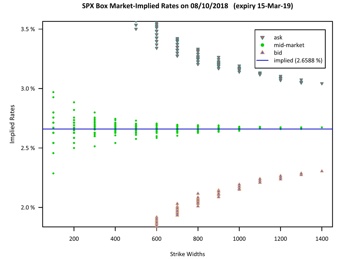
The plot below displays the rates inferred from all possible combinations of box quotes from the NBBO leg markets, where “ask” refers to the rate implied by the box price obtained by crossing the market to sell a box (selling at a higher rate leads to a lower zero bond price), “bid” refers to the cross-market price to buy, and mid-market refers to the rate inferred from the box prices taken by evaluating all legs at the NBBO mid-market.
- Note: The box markets are tighter when traded as outright spreads, but the principle is the same.
Accessing the Interest Rate Term Structure
Once the zero-coupon bond prices have been calculated for the above curves, they are converted into discount factors (i.e. 𝑃𝑎𝑟=1), and the log discount factors are interpolated using a monotone cubic spline to obtain discount factors for the points on the fixed-term grid (in days):
[1, 7, 30, 61, 91, 182, 365, 548, 730, 1095, 1825]
The gridded discount factors are then expressed in SRSE as continuously compounded rates using an Act/365-day count.
Within the SpiderRock Connect trading platform, the fixed term grid is interpolated on log discount factors (i.e. rate * time) using a natural cubic spline.
Observations
All rates are stored using an Act/365-day count convention but are interpreted in the platform using SpiderRock Vol Time. We could convert the rates to a SpiderRock Vol Time day count, but the difference in pricing would likely be negligible.
No swap rates are considered in the LIBOR and OIS term structures since most option expirations are shorter than 2 years
References
Burghardt, G. (2003). The Eurodollar Futures and Options Handbook. McGraw Hill.
Coleman, T. S. (2017, March 9). Comparison of One-Year Swap vs One-Year Libor. Chicago, IL. Retrieved from https://bit.ly/2OtWxZ1
Hull, J. C. (2002). Options, Futures, and Other Derivatives (5th ed.). Prentice Hall.