Option Pricing

SpiderRock Connect's trading platform includes a family of proprietary pricing models that are used to compute prices, implied volatilities, common option greeks (delta, gamma, theta, vega, rho, and phi), and various scenario risk slides for equity and futures options. These pricing models are used in many contexts throughout the platform, including the live servers, GUI tools, and SRSE proxy tables. This document provides an overview of these pricing models and related topics.

Generalized Black-Scholes

SpiderRock Connect's pricing models are solutions (sometimes numeric) to the standard generalized Black-Scholes equation (Haug, 2007):

$\frac{δV}{δt} + \frac{1}{2}σ^2S^2\frac{δ^2V}{δS^2} + (r-q)S\frac{δV}{δS}0-rV=0$

where 𝑉(𝑆,𝑡) is the price of a derivative as a function of stock price S and time t, the variables r and q are the risk-free rate and dividend rate, respectively, and σ is volatility. The equation was originally introduced to price stock options but can be extended to price options on other underlying instruments as well.

The volatility input is not directly measurable, so any pricing solution to this equation is implemented alongside a corresponding inverse function for volatility, known as the implied volatility function.

Within SpiderRock Connect, each solution to the differential equation is implemented in the following functional forms:

$OptionPrice = PriceFunction(ex, cp, strike, uPrc, years, vol, rate, sdiv, dividends)$

and

$Volatility = VolatilityFunction(ex, cp, strike, uPrc, years, opx, rate, sdiv, dividends)$

where

• ex = Exercise type [American, European]
• cp = Option type [Call, Put]
• strike = Option strike price
• years = Years to expiration (see section on Time to Expiration)
• uPrc = Underlying price
• vol = Volatility
• opx = Option price (premium)
• rate = Average discount rate to expiration
• sdiv = Average continuous stock dividend rate to expiration
• dividends = List of discrete dividend payment dates and amounts.

The general form of this equation has several regions of interest. Some regions can be priced using fast closed form solutions (e.g. European calls with no dividends and sdiv = 0), and other regions allow pricing with other analytical methods that are very accurate (e.g. American puts with no dividends and fewer than 2 weeks to expiration). There are also cases that require more complex and significantly slower numerical methods to accurately compute solutions (e.g. American puts with non-trivial discrete dividends).

To address these different pricing situations in practice, the SpiderRock general pricing model is a patchwork of distinct sub-models for a variety of regions of interest. Whenever a closed form solution exists for a region, it will be used. Otherwise, an appropriate numerical method will be chosen. Note that most numerical methods offer only approximate solutions and usually feature a trade-off between accuracy (number of tree steps, grid size, etc.) and computational time (number of calculations per second). SpiderRock Connect typically targets numerical model accuracy that works out to around 1/10th of the minimum price variation in the market in question. However, it is impossible to guarantee this level of theoretical accuracy for all options all the time.

As an example, consider the convergence plot below for a tree calculation of an OTM put option on a stock with an sdiv of 1.25%. For price comparison purposes, the benchmark price of the option is calculated with a 10,000 step CRR binomial tree (Cox, Ross, & Rubenstein, 1979), and the SpiderRock pricing model is used to calculate the option price across a range of tree steps. The plot shows the decrease in pricing error (relative to the benchmark) of a tree calculation as the number of time steps is increased. The same calculation is also shown for a standard CRR tree across the same range of time steps.

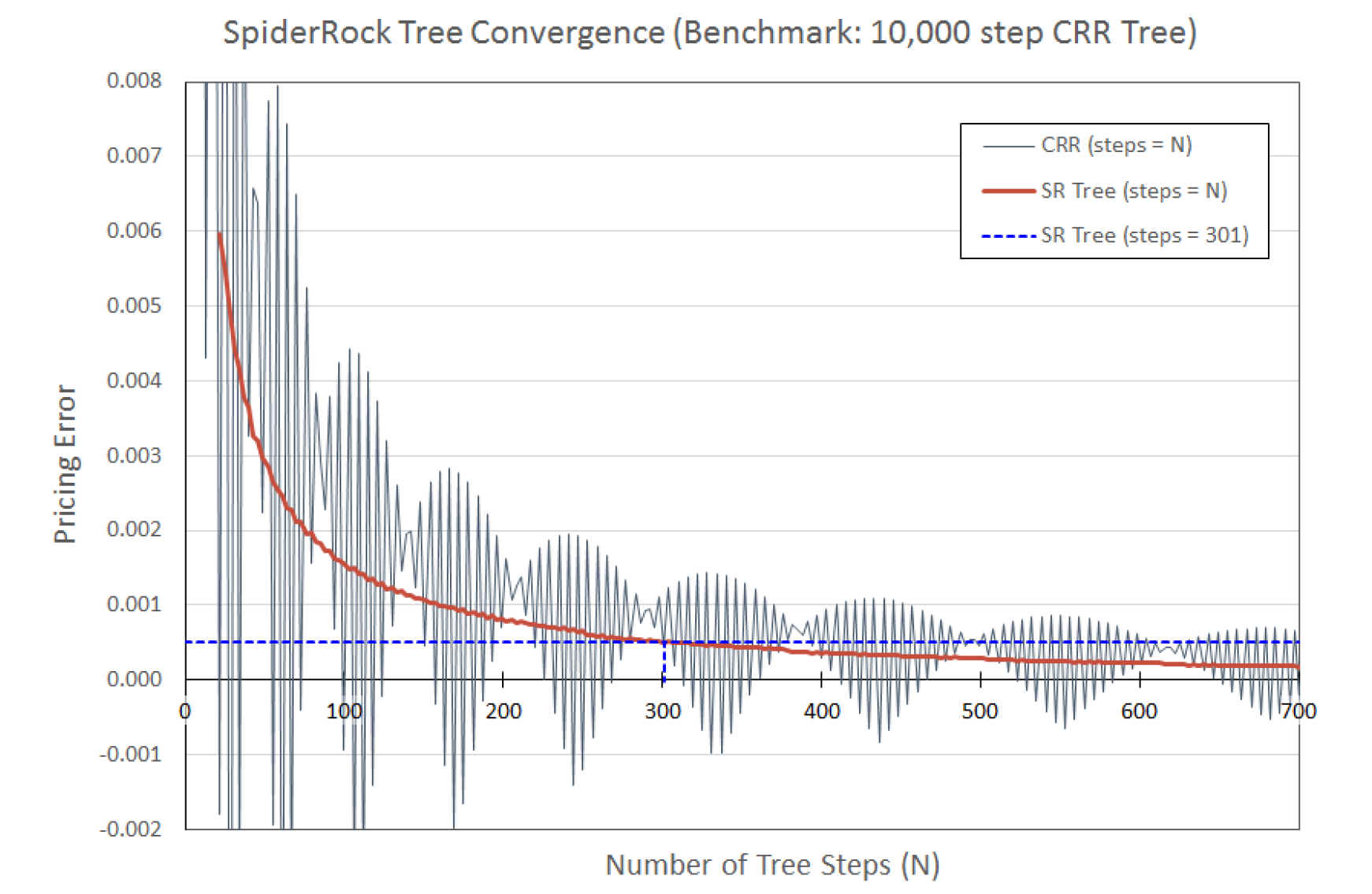
For this specific set of market inputs, the SpiderRock pricing model will use a tree with 301 time steps. Note that the pricing error is roughly half of $0.001, which is well below the stated accuracy goal of 1/10th of the minimum price variation (assuming a minimum tick increment of 0.01). Moreover, the convergence is significantly better than that of the basic CRR tree, which would require more than twice the number of steps to achieve similar results.

The SpiderRock pricing models have been tested and calibrated to known accurate (but slow) models as well as to the published academic literature and are suitable for precise pricing and trading of all listed options. Our core pricing models have been in use for many years and have held up well in a variety of markets.

In practice, accurate pricing and trading of options requires both high-quality pricing models and precisely defined inputs. Differences between values computed from one trading system to the next can often reflect differences in the inputs rather than differences in the choice and implementation of pricing models. Some inputs are universally the same (e.g. cp, strike, vol, opx). Others are precise, but there can be differences depending on implementation (e.g. uPrc can use mid-market, opposite side, weighted average, latency, etc.). The interest rate inputs, rate and sdiv, can require interpolation or estimation from other markets, and they also depend on how a system represents the passing of time. Moreover, both rates and volatilities are expressed in time-dependent units. Discrete dividends, which can require projection from historical payment patterns, also generate differences when the dividend times and/or amounts are not the same between systems.

SpiderRock Connect's trading platform, by default, attempts to make appropriate choices for all inputs and can be used as-is without concern in most reasonable actively traded markets. Note that it is possible, in many but not all contexts, to override the default inputs supplied by the platform.

Underlying Price

SpiderRock Connect defaults to using the current (live) underlying price. The underlying price is usually taken to be mid-market for markets less than 5 ticks wide and the last print (or bid/ask if print is outside of current bid/ask) for wider markets.

When working orders, it is also possible to choose the opposite side of the underlying market (the bid or offer). This is done by picking one of the ‘X’ limit variants (eg. DeX, VolX). The platform will determine which direction you need to trade in the underlying market to hedge the option you are buying or selling, and it will price options under an assumption that you will need to cross the underlying market to hedge.

It is also possible in the SymbolViewer to override the current live market price with any price by specifying it as an override.

Platform Defaults

uPrc: Mid-market (tight markets) or last print (wide markets).

Dividend, Interest, and Carry Rates

The generalized Black-Scholes model involves 3 interest rates: risk-free rate (rate), dividend rate (sdiv), and carry rate (carry). They are related via the formula:

$carry = rate - sdiv.$

This relationship between rates means that the generalized Black-Scholes pricing model depends on only two interest rates, since any of the three rates can be expressed in terms of the other two. Typically for equity pricing, as is the case with SpiderRock Connect, the inputs are entered in terms of rate and sdiv.

The risk-free rate determines how to value cash flows at any given point in time. For option evaluation, it can be viewed as the rate used to discount the future expected payout. The carry rate relates to the expected value of the underlying asset in the future. Under the simplest of assumptions (no dividends and not hard-to-borrow), the carry rate is equal to the risk-free rate for equity options. This can change, for example, when there are discrete dividends to be paid in the future, and the market prices don’t line up with the estimated dividend times and/or amounts in place.

For futures option pricing, the carry rate is set to zero (as with the Black-76 model). In SpiderRock Connect, this is accomplished by setting sdiv equal to rate.

Platform Defaults

Equities:

• rate = Term rate interpolated from risk-free rates
• sdiv = Option-market implied rate (see section on Dividend Rate Calibration)

Futures:

• rate = Term rate interpolated from risk-free rates
• sdiv = rate

For more information, please read our technical note on Interest Rate Term Structure.

Discrete Dividends

The SpiderRock pricing models use a numerical method (modified binary trees w/splicing) to price options with discrete dividends for American calls and puts (Vellekoop & Nieuwenhuis, 2006). This method is accurate for both small and large dividend values, and while it is slow in absolute terms, it is relatively fast compared to other reasonably accurate alternatives.

SpiderRock Connect includes estimates of future dividend dates for all equities that are known to be dividend-paying. If a company has announced a future dividend date or amount, the announced values will typically be used. In addition, for companies that regularly pay dividends, estimated payment dates and amounts will be used to supplement any announced dividends.

The default discrete dividend streams currently in use for pricing options in the platform can be accessed via the SRSE/SRAnalytics table msgSRDiscreteDividend.

It is also possible to override discrete dividends in the SymbolViewer by double-clicking on the dividend panel. However, such overrides only apply to calculations performed in the SymbolViewer, as well in any volatility limit orders generated from the SymbolViewer. These local (per-user) overrides will not affect risk or other calculations performed by background servers.

In addition, discrete dividend overrides can be supplied for individual parent orders when uploading orders via SRSE.

Dividend Rate Calibrations

SpiderRock Connect continuously calibrates call and put implied volatilities for expirations by adjusting the sdiv pricing parameter to minimize the mismatch between call and put surfaces for each individual expiration. This results in an implied sdiv value being computed for each option expiration with reasonable public markets.

This implied parameter can be interpreted as either a market-based correction to a discrete dividend estimate or as an implied estimate of the hard-to-borrow (HTB) rate of the underlying security or both.

Most equity securities that are considered general collateral can be borrowed or lent at the overnight risk-free rate (± borrow fee). If a security goes hard-to-borrow then the borrow fee typically increases from the small general collateral value to a (potentially) much larger value. This has the same effect on cash flows as a nightly dividend (percentage of the underlying price) paid or received when holding or lending the underlying security. As a result, we treat this effective cash flow as a continuous stock dividend (sdiv) in our option pricing models.

Note that most clearing firms quote an overnight HTB rate for securities that go hard-to-borrow. This rate is related to the sdiv rate via the formula:
sdiv = Overnight Rate - HTB Rate.

As the HTB rate gets smaller and becomes more negative, the sdiv rate gets larger and becomes more positive. Also, the sdiv for a general collateral with a borrowing rate of 0% would also be expected to be 0%. In effect, the sdiv rate can be thought of as a measure of how much harder to borrow any given security has become versus the general collateral rate.

The HTB rate quoted by most clearing firms is the overnight HTB rate and is usually good for one day only. This rate, of course, is subject to change over time and may or may not reflect the average expected HTB rate to option expiration. Implied sdiv values, on the other hand, are computed for each individual expiration and (in the case of no or accurate discrete dividends) reflect the average or expected borrow rate to that expiration date.

Note that high short-term HTB rates often revert to more moderate rates over time and that this effect is typically observable in implied market sdiv rates across option expirations.

Also, indexes such as the SPX that have many components that themselves pay dividends can be treated as paying a continuous dividend rather than a large series of discrete dividends. In these cases, the estimated implied sdiv values represent the expected cumulative average dividend payment stream to expiration rather than a HTB rate or an actual continuous dividend rate, and the net effect on the underlying is a decrease in the expected forward price of the index.

Example

By looking at differences between the implied call and put volatilities, it is possible to solve for an implied forward underlying price. SpiderRock Connect's pricing engine will automatically adapt to the market consensus of the forward price by calibrating the sdiv input so that the near ATM implied volatilities match between calls and puts.

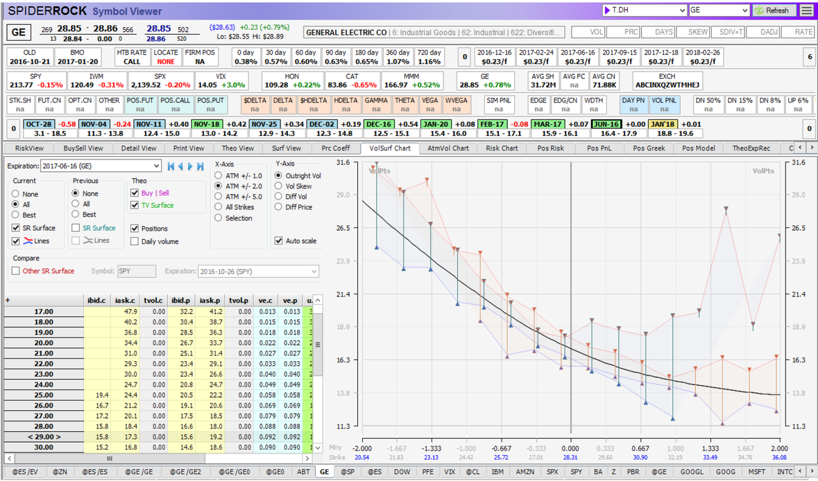
As an example, consider the above snapshot of the June 2017 volatility surface, taken in October 2016.

By adjusting the sdiv input in the upper right-hand corner of the tool, it is possible to demonstrate the impact of a change in the input sdiv rate to the implied volatility markets.

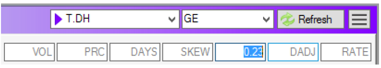
At the time of the market snapshot, the sdiv was calibrated to 23 basis points. The following graphic demonstrates the effect of a 50-bp adjustment up and down from that level:

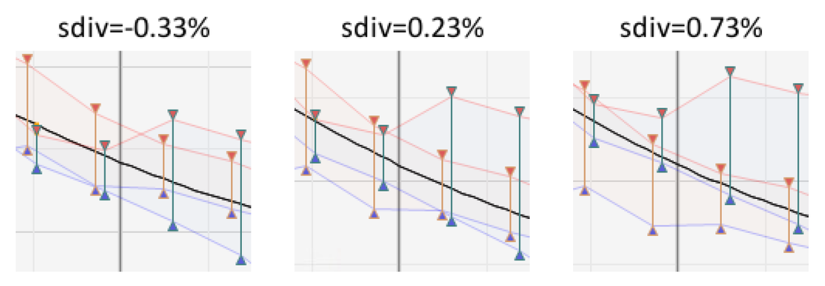
Note that the call and put markets are misaligned on either side of the calibrated 23-bp level.

Over the course of the trading session, the sdiv input is continuously adjusted to keep ATM implied volatilities in line. Generally, the rate level is stable, but it can and will change as the markets move. When the sdiv is small, as in this example, it can be considered as a slight adjustment to account for uncertainties such as the ones mentioned above. In this particular example, the adjustment is small, as evidenced by the dollar value implied by applying the sdiv interest rate to the underlying price and option time to expiration.

$Forward \space price \space adjustment = S \times (1-e^{sdivT})$ $= 28.85 \times (1- e^{0.0023 \times \frac{160.7}{252}})$ $= 0.0423$

Note the resulting 4.2-cent adjustment is relatively small, especially considering that the dividends paid to expiration are estimated at 3*23=69 cents.

Time to Expiration

When an interest rate is established, it includes an assumption of day count, or rather, the convention used to measure time. This same concept is also integral to volatility. If an option is priced using a 365-day convention, the volatility implied from the market will be different than when the pricing model uses a business day count convention. The time convention in place also affects the amount of theta decay that occurs both during and in-between market hours.

When a trading system is configured to use a business day calendar convention, the time-to-expiration only decays during market trading hours, whereas in between each trading day, during holidays, and over weekends, no time can elapse. In prior versions of SpiderRock Connect's trading platform (v6 and earlier), a business day count convention was used. The rule-of-thumb for calculating time was to start with the number of days left to expiration (including the current day) and subtract the fraction of the trading day that had elapsed since the market opened. This fraction was easily calculated by taking the number of trading hours that had occurred since 8:30 AM EST and dividing by the 6.5 hours in a typical US equity market trading day.

This approach oversimplifies the relationship between the underlying price movement during the trading session, and after the market is closed. It assumes that no volatility occurs unless the market is open, and it ignores the possibility that a contract might have trading activity outside of these hours.

Alternately, a continuous, constant-rate time could be employed, where time ticks down minute by minute, at a constant rate, regardless of whether the market is open or closed.

However, neither approach fits the market conditions well. There is observable price volatility that occurs in between market hours, so applying a naïve business day count convention is not consistent when comparing end-of-day volatility with opening volatility during the following trade window. Further, the measurable volatility in between trading sessions is observed to be less than the volatility during market hours, so applying a constant time clock that treats open market hours and closed market hours as equal, will similarly be inconsistent.

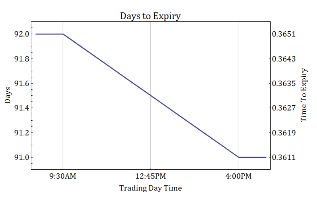
The latest version of SpiderRock Connect (v8 and higher) applies a hybrid time convention that takes both observations into account. During market hours, time is weighted more heavily. In other words, time decays more rapidly during trading hours than it does during overnight and weekend hours. Every minute of the day is treated differently, depending on whether the market session is open or closed, and the resulting time is used in conjunction with volatility.

One minute during trading hours does not amount to the same fraction of a year as a minute during non-trading hours. Time is accounted for, minute by minute so that it is measured in units of years, but the difference in time-to-expiration between two separate moments depends specifically on how many hours are trading hours versus how many are non-trading hours.

Consider an option expiring exactly 48 hours from now, after two consecutive days of trading. For the sake of simplicity, if a trading session is 8 hours long, then there will be twice as much time spent when the market is closed as during market hours (i.e. 16 hours off, then 8 hours on). If the forecast volatility used to price the option is 20%, but 70% of the price variance is expected to occur during the two 8-hour trading sessions, then the time decay can be shifted to make the total variance accrue at a constant rate:

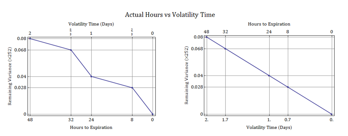
Note that the two plots represent the same relationship between time and volatility. The difference comes from a change in perspective, between the actual hours that pass and the time inferred from an assumption of constant variance. In order to make volatility decay at a constant rate, the “volatility time” needs to reflect the fraction of variance which occurs over each period of time. Simply put, if the non-trading hours generate 30% of the variance, then the volatility time which should elapse over each non-trading period is 0.3 days.

Extending this concept to a business-day count convention for equities, suppose there are 252 trading days, each with 6.5 hours of trading time, representing a total of [2526.5 =1638] hours. Under a 252-trading-day year assumption, the total number of hours in a year is [36524 = 8760] hours, and the remaining non-trading hours in the year amounts to [8760 - 1638 = 7122] hours. If expected volatility is the same between market and non-market hours, each hour should count as 1/8760 of a year.

In this constant volatility framework, the entire year can be broken up into 1638 trading and 7122 non-trading time segments, each representing an hour, all of which add up to 1 year:

$1638 \times \frac{1}{8,760} + 7,122 \times \frac{1}{8,760} = 1$

However, in a business day count convention, where the 7122 non-trading hours account for none of the variance, the time unit used for a single trading hour needs to be adjusted so that the time measured during each trading session accounts for all of the time accumulated in the year. This is accomplished by counting all non-trading hours as equal to zero and counting each trading hour as 1/1638 of a year:

$1638 \times \frac{1}{1,638} + 7,122 \times \frac{0.3}{7,122} = 1$

Any weight can be used to determine the volatility time for a trading hour and for a non-trading hour, by taking a weighted average where α is the percent of volatility attributed to trading time:

$1638 \times \frac{α}{1,638} + 7,122 \times \frac{1-α}{7,122} = 1$

With this approach, we account for time in terms of fractions of hours during trading and fractions of hours outside of trading, each multiplied by their respective volatility “times” for a trading market hour and a non-trading market hour.

$Time \space to \space Expiration = (Trading \space Hours \space Remaining) \times \frac{α}{1,638} + (NonTrading \space Hours \space Remaining) \times \frac{1-α}{7,122}$

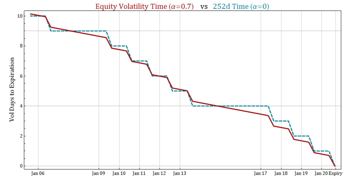
To give an idea of how a 70% trading-time volatility convention (α=0.7) compares against the original 252-day convention in previous versions of SpiderRock Connect (α=0.0), the following plot shows both approaches applied to the last two weeks leading up to the 20 January 2017 expiration. For ease of comparison, the time has been converted into volatility “days” by multiplying time by 252.

Option Greeks

Delta

Delta (Δ) measures the rate of change of the option price with respect to a 1 point change in the underlying price. For analytic and approximation models, the greek is calculated analytically, and for numerical models, the calculation is performed alongside the price calculation, for example, within the same binomial tree used to calculate the option price.

Gamma

Gamma (Γ) measures the rate of change of the option delta with respect to a 1 point change in the underlying price. It is a second-order derivative of the option price with respect to the underlying. For analytic and approximation models, the greek is calculated analytically, and for numerical models, the calculation is performed alongside the price calculation, for example, within the same binomial tree used to calculate the option price.

Vega

Vega measures the rate of change of the option price with respect to a 1% change in volatility. For analytic and approximation models, the greek is calculated analytically, and for numerical models, the calculation is performed by recalculating the option price at 1% increments both up and down and evaluating the slope via a centered difference.

Theta

Theta (θ) measures the rate of change of the option price with respect to a 1-day change in time to expiration. It is always measured numerically, by calculating the difference between the current option price and the option price calculated with volatility time decreased by 1/252 years. For analytic and approximation models, the calculation is performed through a direct call to the model, and for tree methods, the calculation is performed within the tree. When time to expiration is less than 1 volatility day, the next-day option price is taken to be the payout value of the option at expiration.

The value of theta is reported in terms of decay, that is, its value is reported as a positive value of how much option premium is expected to decay in 1 days’ time. There are special cases when the reported value can be negative, in which case, the option premium will be expected to increase in the future. For example, negative call theta values can occur for large values of sdiv, and they can also be observed when an Ex-dividend date is expected within the next day.

Rho

Rho (ρ) measures the rate of change of the option price with respect to a 1% change in the risk-free rate. For analytic and approximation models, the greek is calculated analytically, and for numerical models, the calculation is performed by recalculating the option price at a 1% higher rate and evaluating the slope via a right-handed difference quotient.

Phi

Phi (φ) measures the rate of change of the option price with respect to a 1% change in the dividend rate. For analytic and approximation models, the greek is calculated analytically, and for numerical models, the calculation is performed by recalculating the option price at a 1% higher rate and evaluating the slope via a right-handed difference quotient.

Pricing Model Performance

The core platform pricing model, while accurate, can be too slow in some regions for common tasks. As a result, we have constructed a distributed pricing solution that has two separate components. First, we continuously compute and broadcast, throughout the platform, a collection of “calibration records” which are computed using our high precision models. These calibration records then allow us to quickly and accurately compute prices, volatilities, and greeks using much faster analytic techniques, while still maintaining high precision and consistent pricing throughout the system. The computation and storage of calibration records occur within SpiderRock Connect's data centers and are typically not visible to users.

This distributed pricing solution is highly accurate for most situations. However, in cases where the pricing inputs are significantly different from the current market environment, SpiderRock Connect will use the high precision models. The typical situation where this occurs is in calculating some risk metrics, such as to market shocks and other scenario calculations.

Note that the Symbol Viewer tool uses the distributed pricing solution as the default method for calculating all prices. There are a few specific situations where it may be desirable to temporarily access the high-precision pricing calculations. For example, if input overrides are entered, such as volatility, adjustments to dividends, or price shocks, using the faster analytics-based approach will no longer guarantee sufficient accuracy of the option prices and greeks. The high-precision models can be accessed in the Symbol Viewer by selecting “Use exact pricing”.

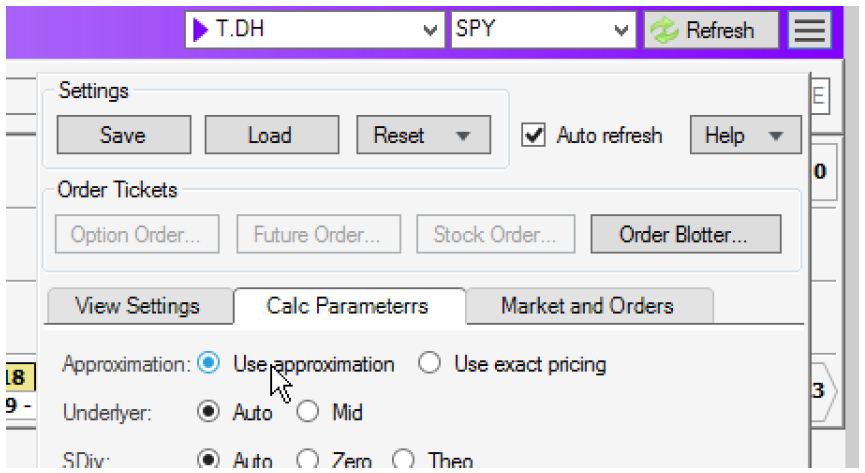
It is important to note that when exact pricing is enabled in the Symbol Viewer, “Auto-refresh” will be disabled. As soon as any input overrides have been cleared, it is recommended to return to the default setting with auto-refresh turned back on.

Root Definitions

All pricing configuration for options is handled by the platform and set at the option root level. These settings can be viewed in the SymbolViewer and via the msgRootDefinition table in SRSE. For example, the following SRSE query lists the types of pricing methods in use:

SELECT root_tk, root_ts, pricingModel FROM srLive.msgRootDefinition;

Currently, there are three pricing methods employed by SpiderRock Connect: ‘Equity’, ‘Future’, and ‘Normal’.

Equity

Equity option pricing uses the generalized Black-Scholes approach described above.

Future

Future option pricing simplifies the pricing problem by always using a combination of the Ju-Zhong model for American options (Ju & Zhong, 1999) and the Black-Scholes closed-form equation for European options. The Ju-Zhong pricing model is an improvement to the approach used by the more well-known Whaley approximation model (Barone-Adesi & Whaley, 1987).

Normal

For pricing options on Eurodollars and other short-term interest rates (STIR), SpiderRock Connect uses an analytic pricing model based on the Ornstein-Uhlenbeck SDE and similar to the equation published in (Iwasawa, 2001).

Other Notes

We automatically switch American options to European on expiration day (there is no early exercise option on expiration day).

We also automatically revert to rate = sdiv = carry = 0 on expiration day, as intraday interest is not typically assessed for most market participants.

It is possible to configure a binary cutoff time (on an account by account basis), after which all hedge delta calculations become binary and take one of the values: [-1, -0.5, 0, +0.5, +1]. If the underlying market is straddling the strike price, a hedge delta of +0.5 or -0.5 is used. Otherwise, for ITM and OTM options, a hedge delta of +1, -1, or 0 is used. The default (which can be changed on request) is that the binary cutoff occurs at 0.5 trading days to expiration.

References

Barone-Adesi, G., & Whaley, R. E. (1987). Efficient analytic approximation of American option values. The Journal of Finance, 42(2), 301-320.

Cox, J. C., Ross, S. A., & Rubenstein, M. (1979). Option pricing: A simplified approach. Journal of Financial Economics, 7, 229-263.

Haug, E. G. (2007). The Complete Guide to Option Pricing Formulas (2nd ed.). McGraw-Hill.

Iwasawa, K. (2001, December 2). Retrieved from http://www.math.nyu.edu/~iwasawa/normal.pdf

Ju, N., & Zhong, R. (1999). An approximate formula for pricing American options. The Journal of Derivatives, 7(2), 31-40.

Vellekoop, M., & Nieuwenhuis, J. (2006). Efficient pricing of derivatives on assets with discrete dividends. Applied Mathematical Finance, 13(3), 265-284.