Client Volatility Surfaces
The purpose of this document is to provide an overview of SpiderRock Connect's volatility surfaces and to describe some of the methods that customers can use to upload their own volatilities into SpiderRock Connect's platform via SRSE.
SpiderRock Connect's surface volatilities are modeled and stored in terms of strike moneyness and volatility percent. This is an approach that normalizes the structure of the curve in a way that is less dependent on the current underlying price and ATM volatility and is more consistent across all strikes and time-to-expiration.
Moneyness
One important concept to understand when modeling volatility is the idea of moneyness. Essentially, it is a relationship between the underlying price and the strike price of an option. When the underlying price (or more specifically, the forward price) is the same as an option’s strike, that option is said to be “at the money”. When the underlying price is either above or below the strike, the option is said to be “in the money” or “out of the money”, depending on whether the option payout would be positive or zero at the underlying price level.
A moneyness function is any increasing function in strike for a given underlying price. Such a function can be useful as a tool to compare relative positions between strikes of different expirations. Two common examples of this are the transformation of strike into standard deviation away from spot and the transformation of strike into put delta. Several moneyness functions can be used for client curves in SpiderRock Connect, and this section defines them.
For sake of simplicity, this document will use the following shorthand symbols or notation:
- S - underlying price, or forward price, depending on modeling requirements
- K - option strike
- T - time to expiration (see the option pricing technical note for an explanation of “volatility time” in years)
- 𝜎𝐴𝑇𝑀 - at-the-money volatility for the option
- 𝜎𝐾 - volatility for an option at strike K
SpiderRock Connect's volatility surfaces are modeled in terms of moneyness instead of strike. This provides for more flexibility and speed when fitting the market because the relative shape of volatility surfaces (for equities and many other products) tends to remain more consistent within this framework. As market underlying prices move around, the shape of volatility can be less variable when viewed in relative terms to the underlying price and ATM volatility.
When strike moneyness is calculated within SpiderRock Connect, the forward of the underlying price is generally used for S, unless otherwise specified.
Standard Deviation
One of the most commonly understood moneyness functions is standard deviation. It is useful both because of its simplicity, and because it evaluates each strike in terms of both volatility and time-to-expiration, allowing reasonable comparisons between different option expirations.
In a typical Black-Scholes framework, volatility can be interpreted in percent terms of the underlying price. An approximation for a single standard-deviation movement in the underlying is given by multiplying the (time-scaled) volatility by the underlying price:
To convert a strike into standard deviation, divide the difference between the strike and the underlying price by a single standard deviation:
- Note: For the above two equivalent expressions, the expression on the left naturally extends from the definition of measuring the distance in terms of a 1-SD move, and the expression on the right reformulates the calculation in terms of percent distance from the underlying price.
Simple
Simple moneyness is a conversion of strike into percent distance from the underlying price:
Simple Root Time
Simple root time moneyness is percent distance from the underlying price, normalized by the square root of time-to-expiration:
- Note: that the similarity to standard deviation moneyness – differing only by a lack of normalization to ATM volatility.
Normal
Normal moneyness is measured by taking the point difference between the strike and underlying price, and dividing by the ATM volatility times the square root of time-to-expiration:
- Note: Normal volatility differs from the more familiar Black-Scholes volatility, in that the units are interpreted in point terms instead of as a percentage of the underlying price level. Thus, a single standard deviation in the underlying is:
With this understanding, Normal moneyness can be interpreted as a standard deviation type of moneyness, as measured by the ATM volatility of a Normal pricing model.
Standard Moneyness
The default moneyness for most curves in SpiderRock Connect is standardized moneyness.
In many respects, standardized moneyness is similar to standard deviation moneyness. The difference is essentially in how the percent distance between the strike and the underlying is calculated. A simple percent-rate calculation comes from the ratio between the strike and the underlying price, whereas a continuous-rate calculation comes from the natural logarithm of the strike to underlying ratio:
One distinct difference between standard deviation and standardized moneyness is that the standard deviation maintains symmetry between strikes of equal distance to either side of 𝑆, whereas standardized moneyness is asymmetric. For a given underlying price 𝑆, the ratio 𝐾/𝑆 is a linear transformation of strike. On the other hand, the expression ln(𝐾/𝑆) is a non-linear transformation of strike, so the strikes that represent a single SD up-and-down move are not equidistant to 𝑆.
Example
Some example calculations are provided in the table below. (S=120, 𝜎=15%, T=0.25)
| Strike | Standard Deviation | Simple | Simple Root Time | Normal (σ=15.0) | Standardized |
|---|---|---|---|---|---|
| 100 | -2.2222 | -0.1667 | -0.3333 | -2.6667 | -2.4310 |
| 110 | -1.1111 | -0.0833 | -0.1667 | -1.3333 | -1.1602 |
| 120 | 0 | 0 | 0 | 0 | 0 |
| 130 | 1.1111 | 0.0833 | 0.1667 | 1.3333 | 1.0672 |
| 140 | 2.2222 | 0.1667 | 0.3333 | 2.6667 | 2.0553 |
- Note: For the Normal moneyness calculation, volatility has been taken to be 15.0 instead of 0.15 (for 15%) to maintain a similar scale for comparison to the other columns.
Percent ATM Volatility
SpiderRock Connect's Surface Volatilities are modeled in terms of percent of the ATM volatility:
When volatilities are encoded in percent volatility terms, they can be recovered by solving for strike volatility:
Example
Consider the following example table of moneyness and percent volatilities:
| Moneyness | Percent ATM Vol | Strike Vol (σ = 15%) |
|---|---|---|
| -1.5 | 0.375 | 20.625% |
| -1.0 | 0.30 | 19.500% |
| -0.5 | 0.15 | 17.250% |
| 0 | 0 | 15.000% |
| 0.5 | -0.05 | 14.250% |
| 1.0 | 0.01 | 15.150% |
| 1.5 | 0.05 | 15.750% |
As before, assume the underlying price is 𝑆=120, and the expiration time is 𝑇=0.25. The corresponding strike volatilities have been entered in the table for the specific case when the ATM volatility is 15%.
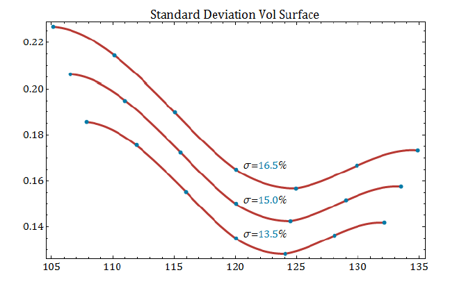
Now let’s consider 3 cases, given by ATM volatility levels of 13.5%, 15%, and 16.5%. Using a standard deviation moneyness convention and applying a spline between points, the volatility surfaces may look something like this:
For sake of comparison, using a standardized moneyness convention with otherwise similar market assumptions results in a slightly different set of volatility surfaces:
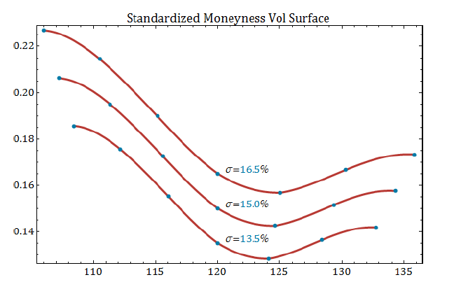
In both plots, the blue points represent strikes corresponding to the uniform moneyness grid 1.5.
Both moneyness examples generate similar surfaces. The volatilities at each moneyness point are the same, by design. However, the two plots are subtly different; for example, note the difference in symmetry. For the first plot, the interval between each moneyness point in strike terms is the same across the surface for each ATM volatility level – uniformly spaced strikes are converted into uniformly spaced moneyness values. However, for the second plot, using standardized moneyness, the lower strikes are generally closer to 𝑆=120, and the upper strikes are successively further away from 𝑆=120.
This distinction can make a difference when fitting markets, depending on the option markets involved.
Volatility Surface Dynamics and Hedging
When non-trivial moneyness transformations are used to model volatility across strikes, the resulting curves exhibit a natural volatility dynamic, because the ATM value (i.e. the zero xAxis value) moves with the underlying price. As a result, all SpiderRock curves slide to the left and right as the underlying changes. In addition, SpiderRock curves are constantly re-pinned to ATM values, frequently enough that our ATM curve values react to changes in market conditions almost instantaneously.
However, the raw model deltas computed from the live instantaneous surfaces volatilities do not account for any surface dynamics. Typically, this relationship is expressed using an “adjusted” delta for each option at each strike, calculated from the raw model greeks:
where
This rate of change can be decomposed into two parts:
The first part relates to how volatility changes at a fixed strike as the moneyness changes, or rather, as the volatility curve moves to the left and right. This is directly measurable from the shape of the curve.
The second part relates to how the ATM volatility in the market moves as the underlying price changes. This rate of change can be measured over time, usually through analysis of market underlying price data and ATM volatilities. For the ICurve and TheoSpline models, the second part can be controlled via the 𝑡𝑣𝑆𝑙𝑜𝑝𝑒 parameter for each uploaded curve:
SpiderRock Connect's hedging tools and account configuration settings allow multiple kinds of hedgeDelta computation. Hedge deltas can be configured to be simple (raw deltas from surface vols), surface adjusted (using the adjusted delta approach), or hedge deltas derived from client theoretical surfaces, expressed either as simple or adjusted deltas.
The current account configurations for SpiderRock hedge deltas are:
- IVol - Delta is calculated from SpiderRock surface (𝑉𝑒𝑔𝑎𝑆𝑙𝑜𝑝𝑒=0). This is the default setting.
- IvS - Adjusted Delta is calculated from SpiderRock surface using a trivial 𝑡𝑣𝑆𝑙𝑜𝑝𝑒 assumption (𝑉𝑒𝑔𝑎𝑆𝑙𝑜𝑝𝑒=𝑠𝑘𝑒𝑤𝑆𝑙𝑜𝑝𝑒).
- TVol - Delta is calculated from client surface (𝑉𝑒𝑔𝑎𝑆𝑙𝑜𝑝𝑒=0).
- TvS - Adjusted Delta is calculated from client surface using the client-defined 𝑡𝑣𝑆𝑙𝑜𝑝𝑒 (𝑉𝑒𝑔𝑎𝑆𝑙𝑜𝑝𝑒=𝑠𝑘𝑒𝑤𝑆𝑙𝑜𝑝𝑒+𝑡𝑣𝑆𝑙𝑜𝑝𝑒).
- TvolAll - All greeks are calculated from a client supported surface.
- TvolAlls - All greeks are calculated from the client supplied Skew adjusted Delta and corresponding client surface values.
Please contact SpiderRock Client Support Desk for assistance in changing the hedge delta rule for an account.
Theoretical Volatility Slope
The theoretical volatility slope (𝑡𝑣𝑆𝑙𝑜𝑝𝑒) is the rate of change of the theoretical ATM volatility with respect to the underlying price. When 𝑡𝑣𝑆𝑙𝑜𝑝𝑒 is non-zero, the ATM volatility input used to define a curve will change as the underlying price moves.
The msgtheoexpsurface table contains fields which provide control over the ATM volatility of a user-defined theoretical volatility curve. As the underlying price changes in the market, the ATM volatility defining any curve can be configured according to the following parameters:
- refUPrc - Reference underlying price which corresponds to the initial input theoVol
- refUPrcWeight - Weight (𝜔) used to determine the relationship between moneyness and the reference underlying price versus the current underlying price. The value is currently enforced to be within the interval [0,1].
- theoVol - Theoretical volatility to use as the anchor for defining the dynamic ATM volatility of the curve
- tvSlope - Rate of change of the ATM volatility, measured in decimal units of volatility per each 1-point change of the underlying
The dynamic ATM volatility (𝑑𝑦𝑛𝑎𝑚𝑖𝑐𝑉𝑜𝑙) for a curve is defined as follows:
Skew Stickiness
Skew stickiness is a term used to describe how the shape of the volatility skew changes relative to each strike as the underlying price moves. Two commonly referred to examples are “sticky strike” and “sticky delta”.
For a sticky strike dynamic, the skew shape tends to remain the same between each strike, regardless of where the underlying price is. This relationship might be observed in the market if, for example, the volatility spread between two different strikes remains fixed as the underlying moves. In this situation, the ATM volatility might vary, but the volatilities would tend to change uniformly across all strikes, moving up or down in parallel.
For a sticky delta dynamic, the skew shape tends to remain the same between the ATM point of the curve and other points on the curve that are a relative distance away from the center. For example, the volatility spread between the ATM strike and the 20-delta call strike might remain the same as the underlying price moves. In this situation, the ATM volatility might also vary, but the general shape of the volatility curve would tend to move left or right in the direction of the underlying price, as it changes.
Each volatility curve is modeled in terms of skew moneyness, and in turn, the moneyness function represents a relationship between option strikes and the market forward underlying price. For example, strikes are sometimes referred to in terms of standard deviations away from the market forward. This relationship between volatility and the underlying price is used to control skew stickiness.
For equities, the forward is calculated as:
The skew stickiness is controlled by varying the rate at which the reference underlying price changes with the market. If the reference underlying price doesn’t change, the moneyness function will also not change. For equities, the reference underlying price passed into the moneyness formula is the weighted average:
where 𝜔=𝑟𝑒𝑓𝑈𝑃𝑟𝑐𝑊𝑒𝑖𝑔ℎ𝑡.
When pricing on futures contracts, the moneyness is calculated using the same approach to weighting, but without calculating the forward, since the underlying is already in terms of the underlying value at expiration.
- Note that when 𝜔=0, the most recent underlying price (𝑢𝑃𝑟𝑐) is used, and when 𝜔=1, the reference underlying price (𝑟𝑒𝑓𝑈𝑃𝑟𝑐) is used for the moneyness calculation. These two cases correspond to sticky delta and sticky strike, respectively.
VegaSlope
VegaSlope is defined as the rate of change of volatility as the underlying price changes. It is reported on an individual strike basis, because it can be a different for each strike. For example, in the plot below, the reference underlying price weight is set to 𝜔=0, and 𝑡𝑣𝑆𝑙𝑜𝑝𝑒 is defined so that there is a decrease in theoretical ATM volatility at a rate of 15-bp for each 1-point increase in the underlying. This corresponds with a sticky delta dynamic.
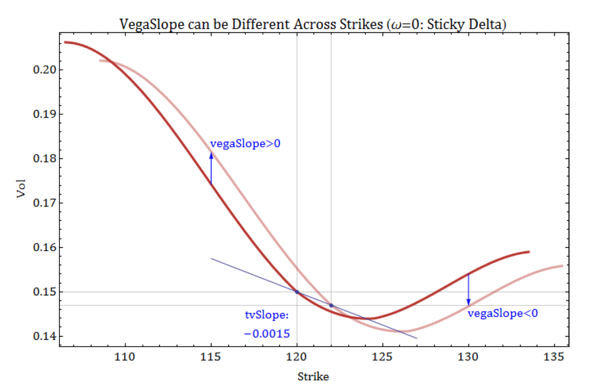
- Note that most of the volatilities increase for strikes below and near the ATM point, and volatilities for strikes above the ATM region decrease when the underlying price increases. However, there are also a few strikes where the volatility does not change when the curve moves. This translates into a range of positive and negative values of vegaSlope across the strikes.
In contrast, when 𝜔=1, the volatility curve follows a sticky strike dynamic. The values of vegaSlope across all strikes tend to be more uniform, because the primary curve movement is vertical, rather than horizontal.
TheoSpline Moneyness (xAxisType)
When a user-defined volatility is defined using the SpiderRock TheoSpline model (described in the next section), there are a few newly added moneyness definitions that allow the user to control whether the convention depends on a dynamic volatility or a static volatility. VolRTMoney was defined prior to V7, and the dynamic volatility version, TVolRTMoney, has been added to V7. Also, static and dynamic versions of standardized moneyness have also been added. The possible choices for xAxisType are:
| xAxisType | Equation |
|---|---|
| Strike | |
| SimpleMoney | |
| RTMoney | |
| VolRTMoney | |
| TVolRTMoney | |
| LogStdMoney | |
| TLogStdMoney |
One key reason for providing the dynamic versions of each type is so that it’s possible to choose a moneyness function that is consistent with the case when refUPrcWeight ω is defined either at 0 or 1. VolRTMoney and LogStdMoney are more consistent with a sticky strike dynamic, because the forward price and the volatility do not change in the formula when the underlying price and ATM volatility move. The axisVol implemented in the moneyness formula is constant, defined by the user along with the other curve shape inputs.
In contrast, for a sticky delta dynamic, it’s more typical to have the shape of the volatility curve “breathe”, or increase in width, as the dynamicVol increases. TVolRTMoney and TLogStdMoney provide this behavior, adapting to each change in both the underlying price and the resulting dynamicVol.
- Note that the TVolRTMoney convention was used for the above sticky strike example plot. Both volatility curves are plotted from -1.5 to 1.5 moneyness, and for the higher volatility curve (i.e. when uPrc=120 and dynamicVol=15%), the covered strike range is slightly wider than the volatility curve generated for uPrc=122 and dynamicVol=14.7%. If the VolRTMoney axis type had been used, the width of the curves would be unchanged as the underlying price moved, and the sticky strike dynamic would lead to a parallel shift in volatility across all strikes.
Uploading Customer Volatilities
msgSRTheoExpSurface
The SRTheoExpSurface table is used to upload customer-defined volatilities. Each option expiration can be assigned a customer-specific volatility surface definition via a selection of different possible surface models. Each entry in the table is keyed by option expiration and by a model account, which is used to link the entries in the table to the appropriate client account. Contact SpiderRock Client Support Desk to determine which model account name to use for any specific client account.
There are several available surface models, which are explained in this section. Note that all models use the dynamic ATM volatility, 𝑑𝑦𝑛𝑎𝑚𝑖𝑐𝑉𝑜𝑙, determined by current market underlying prices along with the user input values of theoVol and tvSlope.
For most of the surface models, the user can define values for refUPrc (𝑆𝑅𝑒𝑓) and refUPrcWeight (ω). The weight, ω, can be set to any value from 0 to 1, and it is used to adjust the ‘stickiness’ of the underlying price S used in the moneyness calculation for each surface. When ω=0, the moneyness is calculated relative to the market forward of the underlying price (uPrc) minus discrete dividends (ddiv) when they exist. Similarly, when ω=1, the moneyness is calculated with respect to the forward of the reference underlying price, 𝑆𝑅𝑒𝑓.
For clients wanting to replicate behavior in SpiderRock V6, use refUPrcWeight=1 and 𝑡𝑣𝑆𝑙𝑜𝑝𝑒=0.
Recall that the general formula for the forward price S used to calculate moneyness is:
In addition to defining the volatility surface model and setting the model inputs, there are additional inputs that can be used to adjust the dividend inputs, and define different volatility curves and edge settings for both buying and selling.
Please contact SpiderRock Client Support Desk for more information on these additional settings.
TheoSpline
Parameters: dynamicVol
SRSE Table: msgsrtheoexp2ptcurve
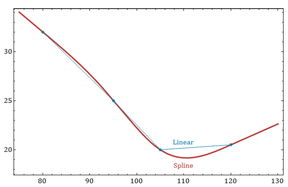
A spline is a polynomial curve fitting method that is defined to return the precisely defined values at the input points (or strikes) and which connect these values with a curve that is reasonably smooth in between the defined points. It is an improvement over simple linear interpolation, which essentially draws a line between each adjacent input strike and follows the line to approximate any values in between strikes. Cubic splines are a commonly used tool for volatility interpolation.
The picture below is an example of a spline curve on 4 points, as it compares with linear segments between the points.
The TheoSpline model enables clients to enter a volatility surface definition via a grid of moneyness points and volatility percentages. The spline knot points are defined in the msgsrtheoexp2ptcurve table, and the curve is interpolated between points using a natural cubic spline. The region outside the strike range is extended linearly, according to the slope of the cubic spline at the outer-most points of the grid.
The xAxisType can be set to any of the supported moneyness conventions described above in TheoSpline Moneyness (xAxisType).
For more information on the msgsrtheoexp2ptcurve table, please contact SpiderRock Client Support Desk.
ICurve
Parameters: dynamicVol, paramA (slopeAdj), paramB (volAdj)
The ICurve model uses the SpiderRock live-fit surface as the initial shape of the volatility surface, and then transforms it according to the user-defined theoVol, slopeAdj, and volAdj. This model provides a simple framework with which customers can manipulate the SpiderRock surface by setting their own user-defined dynamic ATM volatility, applying a tilt (increasing or decreasing the original curve slope), and re-scaling the percent volatilities across the surface (applying a percent adjustment across the original fitted curve).
The resulting curve volatilities at each strike are calculated according to the following formula:
where
- percentVol - Percent volatility from the live SpiderRock surface.
- volAdj - When volAdj is non-zero, the live SpiderRock surface percent volatilities are increased or decreased by a factor of 1+volAdj. Units are in decimal percent. The moneyness for each strike is defined purely in terms of the SpiderRock Live Surface parameters and is not affected by the refUPrc and reUPrcWeight settings.
- slopeAdj - When slopeAdj is non-zero, the surface percent volatilities are increased or decreased by adding a linear shift of slopeAdj*xAxis across the curve. Units are in (percent volatility)/moneyness.
- xAxis - Moneyness value for the SpiderRock surface at any strike.
- Note that when both the slopeAdj and volAdj parameters are set to zero, ICurve is essentially an implementation of the SpiderRock Connect surface shape, where a user-defined volatility dynamic is used instead of the SpiderRock calibration to market ATM volatilities.